A finite element run finishes and the peak equivalent stress sits above yield: 412 MPa against a yield strength of 355 MPa. Whether that calls for reinforcement is not obvious, because the number on screen shifts with mesh density, element type, the shell surface on display, and the averaging setting. The sections below explain how to identify the equivalent stress value that actually belongs in a code check.
What the formula collapses?
Six components describe the stress state at a point. The von Mises criterion reduces them to a single scalar using only the deviatoric part of the tensor, the part tied to change of shape.
The hydrostatic part, which drives change in volume, drops out of the calculation entirely. Written out in full through tensor components, the plane stress form reduces to σ_VM = √(σx² + σy² − σx·σy + 3τxy²).
Take biaxial tension with σx = 200 MPa, σy = 150 MPa, and no shear. The equivalent stress comes out at 180.3 MPa, 9.9% below the maximum principal stress of 200 MPa.
The number on screen is lower than the actual peak at that point, and that is correct. The criterion describes the onset of yield, and it coincides numerically with the principal stress only in the uniaxial case.
Von Mises stress is always non-negative and does not indicate whether the underlying stress state is tensile or compressive.
Peak values follow the mesh
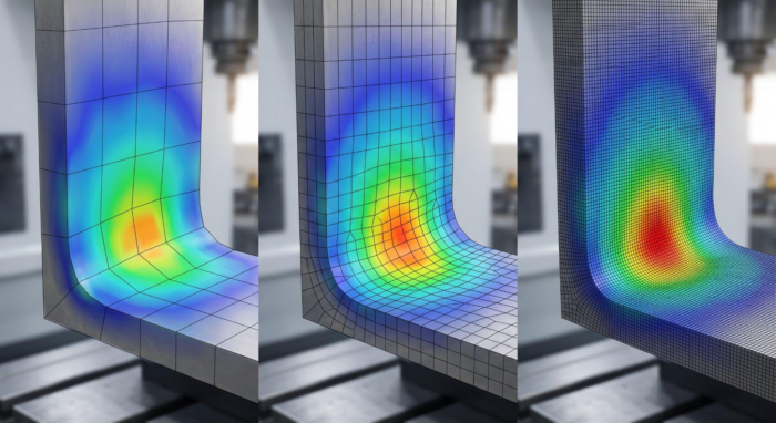
Accuracy tracks discretization. Refining the mesh inside a stress concentration produces a converging sequence: a 10 mm element gives 85 MPa, 5 mm gives 97 MPa, 2.5 mm gives 101 MPa, 1.5 mm gives 102 MPa. The increments run 14.1%, then 4.1%, then 1%. That final step is what convergence looks like.
Formal convergence assessment relies on the grid convergence index, which expresses the difference between successive refinements as an uncertainty band. On a well-refined elastic mesh those values stay under 2%, and they widen once plasticity enters the model.
A coarse mesh understates the peak. At 85 MPa against a converged 102 MPa, the shortfall is 16.7%. Where the utilization factor sits near unity, an error of that size can confirm a capacity that is not there and record a margin that does not exist.
When refinement produces no convergence at all, the usual cause is a stress singularity. Geometric idealization is the common source, and the computed peak then climbs without limit.
Averaged and unaveraged values
Stresses are solved at integration points inside each element and then extrapolated to the nodes. A node shared by four elements therefore receives four separate values.
Node averaging displays their arithmetic mean and produces a continuous contour. With averaging switched off, the discontinuities between adjacent elements become visible.
A wide spread between the contributions at a shared node points to a mesh too coarse to capture the local gradient. Averaging can conceal that condition, since a smooth plot suggests a converged solution on a model that has not converged. Comparing both display modes gives a read on mesh quality that does not depend on any formal convergence criterion.
A shell has three surfaces
Shell elements carry stresses on the top, bottom, and mid-surfaces. The difference between them comes from bending through the thickness. The decomposition is standard: membrane σm = (σtop + σbottom)/2, bending σb = (σtop − σbottom)/2.
At a point with a membrane component of 50 MPa and a bending component of 80 MPa, the top surface reaches 130 MPa, and the bottom surface sits at minus 30 MPa. Averaging the two von Mises readings already computed, 130 and 30, returns 80 MPa. That overstates the actual membrane stress of 50 MPa by 60%.
The error is one of sequence. The von Mises stress formula applies to stress tensor components, so averaging through the thickness has to happen on those components before the equivalent value is computed. Von Mises scalars have already lost their sign, which puts the compressed surface on the same footing as the tensile one.
Viewing a single surface leaves half the field out of sight. Under bending-dominated loading, the true maximum often sits on the face that is not currently displayed.
What the code does with the number?
EN 1993-1-1 clause 6.2.1(5) sets out the yield criterion in normalized form: each stress component is divided by the design resistance fy/γM0, and the result of Formula 6.1 is capped at unity.
For a point with a longitudinal stress of 220 MPa, a transverse stress of minus 40 MPa and a shear stress of 95 MPa in S355 steel with γM0 = 1.0, the equivalent stress reaches 293 MPa, a utilization factor of 82.5%.
Checking the longitudinal stress alone returns 62%. The 20.5 percentage point gap comes from the shear and transverse components that a one-dimensional check leaves out.
The code also limits where this criterion applies. Elastic verification at a point is conservative because it excludes the partial plastic redistribution that elastic design permits, so it is intended for cases where direct cross-section resistance checks through NRd, MRd and VRd cannot be applied.
Stress extraction rules vary between code systems as well. DNV-RP-C201 builds its plate yield check on membrane stresses, while Formula 6.1 of EN 1993-1-1 imposes no such restriction, which means the same physical stress state can be assessed differently depending on which standard governs the project.
Since 2025, finite element design has had its own part of the Eurocode. EN 1993-1-14, “Design assisted by finite element analysis,” consolidates rules that previously sat in informative Annex C of EN 1993-1-5, and it separates two verification routes.
On the first, the model returns internal forces and stresses that are then checked against the ordinary EN 1993 equations. On the second, the model returns the resistance directly and carries its own model factor γFE.
Both routes share one requirement: verification and validation of the model are performed and documented, with the credibility of the result established quantitatively.
Where the criterion answers a different question?
Fatigue assessment works on different principles. Crack growth is driven by the range and direction of the principal stresses, while the von Mises equivalent stress carries no directional information and never goes negative. EN 1993-1-9 and DNV-RP-C203 assess fatigue through the stress range Δσ against S-N curves.
Feeding an equivalent stress into that framework produces numbers that do not correspond to the endurance curves they are compared against.
Welded connections follow their own rules. The directional method in EN 1993-1-8 takes the stress components on the weld throat section and applies the criterion √(σ⊥² + 3(τ⊥² + τ∥²)) ≤ fu/(βw·γM2), with σ⊥ ≤ 0.9·fu/γM2 as an additional condition.
The mathematical resemblance to von Mises is genuine, but the inputs and the resistance being compared against are different.
Equivalent stress says nothing directly about stability either. Thin-walled members can buckle at stresses well below yield, which calls for a dedicated stability analysis.
For brittle materials such as concrete and cast iron, and for composites, the hydrostatic part of the tensor that the criterion discards plays a substantial role in failure, so other strength criteria apply.
Reading the result in order
An equivalent stress field is an intermediate result of the analysis. Before a peak value is compared against a design resistance, it has to be qualified on four counts: whether the mesh has converged, which averaging mode is active, which shell surface the maximum was taken from, and what form of check the governing code requires.
Working through those four points separates a physically meaningful result from a post-processing artifact. Without that control, peak values carry no demonstrable credibility and become difficult to defend under independent review.